Post 1 of 2: implement the green-red list watermark, detect it with a proper statistical test, and measure what it costs.

📝 Notebook

In August 2026 Anthropic announced that new Claude models will watermark the text they generate, using a version of Google DeepMind's SynthID-Text (TechCrunch). Google has watermarked Gemini text with SynthID-Text since 2024 (Dathathri et al., Nature, 2024). The transparency rules of the EU AI Act are one of the drivers. Text watermarking has moved from research papers into production systems.

In this series we build a text watermark from scratch with the method that started this line of work: the "Green-Red list" method of Kirchenbauer et al. (2023), A Watermark for Large Language Models. SynthID-Text belongs to a related but different branch. Kirchenbauer's method shifts the model's probabilities toward some tokens. SynthID-Text keeps the probabilities and instead replaces the source of randomness used to sample from them (tournament sampling), which is how it avoids hurting text quality. Both share one core idea: a secret key plus the recent context decide, pseudo-randomly, which choices carry the mark. We will cover SynthID-Text in some next post.

Roadmap

This first post covers:

1. Baseline. Implement the method with a one-token context, look at the watermark token by token, and see why a naive detection rule fails.

2. Statistics. Turn detection into a proper hypothesis test: z-score, CLT, p-values.

3. The knobs. How the bias δ, the green fraction γ and the model's entropy trade text quality against detectability.

The second post continues with:

1. Attacks. Build one evaluation harness with three kinds of edits, from random noise to a full LLM paraphrase.

2. Context schemes. Change only the rule that turns context into a seed, run every variant through the same harness, and measure the robustness-versus-security trade-off.

3. Limitations and outlook.

Every comparison in this series uses the same prompts, random seeds, sampling settings, text length, γ and δ, so any difference you see comes from the one thing we changed.

The code in this post shows only the key parts; everything else is replaced by short comments. The full, runnable code is in the companion notebook.

How the green-red list watermark works

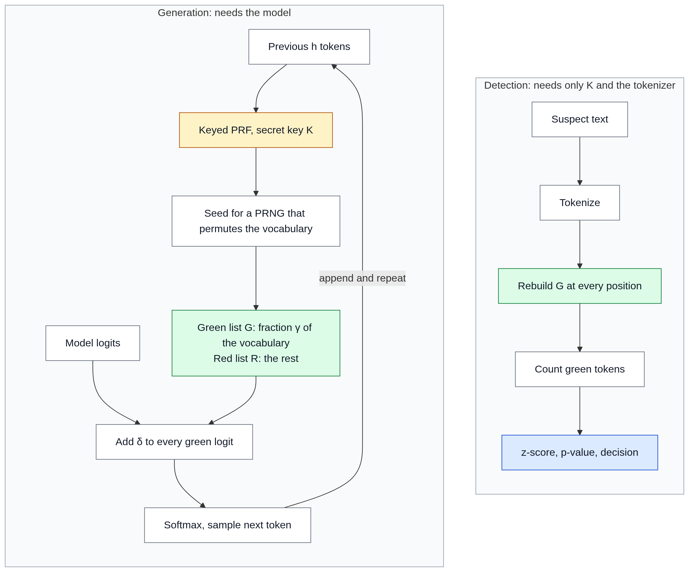
Notation. V is the vocabulary, \(s_t\) the token at step t, \(l_k\) the model's logit for token k, h the context width, K the secret key.

Step 1: Partition the vocabulary

Before the model picks token \(s_t\), the algorithm looks at the previous h tokens (\(h=1\) in the basic version of the paper). A keyed pseudo-random function turns that context into a seed:

$$\text{seed}t = \mathrm{PRF}K(s{t-h}, \dots, s{t-1})$$

The seed drives a pseudo-random number generator that shuffles the vocabulary. The first \(\gamma|V|\) tokens of the shuffle form the green list \(G_t\); the rest form the red list \(R_t\). The hash function and the PRNG can be completely public. Only the key K is secret: anyone who has it can recompute every green list; anyone who doesn't sees ordinary text. Because the seed depends on the context, the partition changes at almost every step. Common choices are \(\gamma = 0.25\) or \(\gamma = 0.5\); we use 0.5.

Step 2: Shift the distribution

The model produces a logit for every token. Before the softmax, the algorithm adds a constant \(\delta\) (the watermark strength) to the logit of every green token:

$$\tilde{\ell}_k = \begin{cases} \ell_k + \delta & \text{if } k \in G_t \ \ell_k & \text{if } k \in R_t \end{cases} \qquad\Longrightarrow\qquad \tilde{p}k = \frac{e^{\ell_k + \delta,\mathbb{1}[k \in G_t]}}{\sum{j \in V} e^{\ell_j + \delta,\mathbb{1}[j \in G_t]}}$$

Red tokens are not forbidden. The paper first presents a hard rule that bans red tokens completely, then replaces it with this soft rule, because banning tokens destroys text whenever the only sensible next token happens to be red. With the soft rule, a red token still wins whenever its logit is more than \(\delta\) above the best green one.

Why a soft shift works. When the model is very confident (low entropy: one token holds almost all the probability), a red token with a much larger logit than every green token still gets picked with high probability. The watermark steps aside and the text stays correct. When the model is uncertain (high entropy: several synonyms are about equally likely), the bias tilts the choice toward the green synonym. The watermark therefore lives in the high-entropy positions of the text.

The trade-off. Two goals pull against each other: fluency (don't override the model's preferred word) and detectability (put as many green tokens in the text as possible). In the best case for the watermark, a position where the model's probability is spread evenly, the chance of picking a green token is

$$P(\text{green}) = \frac{\gamma e^{\delta}}{\gamma e^{\delta} + 1 - \gamma},$$

which for \(\gamma = 0.5\) is about 73% at \(\delta = 1\), 88% at \(\delta = 2\) and 98% at \(\delta = 4\). At low-entropy positions it stays close to what the model wanted anyway. A larger \(\delta\) gives stronger evidence per token but overrides the model more often, so quality drops. Low-entropy text (code, facts, lists) carries little watermark whatever \(\delta\) we choose. Part 3 measures both effects.

Step 3: Detect

The detector needs the key and the tokenizer, not the language model. It re-tokenizes the suspect text, rebuilds \(G_t\) at every position from the preceding tokens, and counts how many tokens are green. In text written without the key, each token lands in its green list with probability \(\gamma\), so about half of them are green. Watermarked text has too many green tokens. Deciding how many is "too many" is a statistics question, and Part 2 answers it.

Setup

pip install "transformers>=5.0" torch nltk scipy pandas matplotlib

Generation dominates the runtime. On a GPU the whole companion notebook runs in minutes; on a CPU a 2B model is much slower, so start with QUICK_RUN = True. Generations are cached on disk (CACHE_DIR), so re-running a plotting cell never regenerates text.

# Imports: hashlib, math, random, numpy, pandas, torch, matplotlib, nltk,
# scipy.stats (norm, binom, binomtest) and, from transformers,
# AutoModelForCausalLM, AutoTokenizer, LogitsProcessor, LogitsProcessorList

MODEL_NAME = "openbmb/MiniCPM5-2B"
SECRET_KEY = b"replace-with-your-own-key"   # the ONLY secret of the scheme (max 64 bytes)
SEED = 1234

GAMMA = 0.5                # green-list fraction, fixed in every comparison
DELTA = 2.0                # watermark strength, fixed in every comparison (Part 3 sweeps it)
Z_THRESHOLD = 4.0          # one-sided p ≈ 3.2e-5
MIN_SCORED_TOKENS = 16     # below this we refuse to decide

# Pure multinomial sampling, as in the paper. The watermark processor runs *before*
# temperature / top-p in transformers, so with temperature T the effective bias is δ/T.
SAMPLING = dict(do_sample=True, temperature=1.0, top_p=0.95, top_k=0)

# Experiment sizes: 10 prompts, 200 new tokens per text, 50 human texts, 3 long texts of 500 tokens
# (plus a QUICK_RUN switch, the disk cache, BATCH_SIZE and device selection; see the notebook)
PROMPTS = [
    "The future of artificial intelligence will bring",
    "The history of the printing press shows that",
    "Coffee has been part of daily life for centuries because",
    # ... 10 open-ended prompts in total
]

tokenizer = AutoTokenizer.from_pretrained(MODEL_NAME)
model = AutoModelForCausalLM.from_pretrained(MODEL_NAME, dtype=DTYPE).to(DEVICE).eval()

# The watermark must use the size of the logit vector, which can differ from len(tokenizer)
VOCAB_SIZE = model.get_output_embeddings().weight.shape[0]
# (plus the padding token and end-of-sequence ids needed for batched generation)

for pkg in ["wordnet", "omw-1.4", "brown", "stopwords", "averaged_perceptron_tagger", "averaged_perceptron_tagger_eng"]:
    nltk.download(pkg, quiet=True)

NLTK data packages: what we need them for

The nltk library ships only code; corpora, word lists and trained models are separate data packages. The loop above downloads them once into a local folder (usually ~/nltk_data) and skips packages that are already present.

Package	What it is	Used for
brown	The Brown corpus: about one million words of American English from the 1960s	Human-written texts for the null distribution and false-alarm tests (load_human_texts)
wordnet	A dictionary of English words grouped into synonym sets	Both word-replacement attacks (wn.synsets, lemma names)
omw-1.4	Open Multilingual WordNet, extra data that accompanies WordNet	Not used directly; some NLTK versions expect it next to WordNet
stopwords	Lists of very common words ("the", "is", "of")	The synonym swap skips these words
averaged_perceptron_tagger_eng	A trained part-of-speech tagger	nltk.pos_tag in the synonym swap, which only replaces singular nouns, adjectives and adverbs
averaged_perceptron_tagger	The same tagger under its pre-3.9 name	Compatibility with older NLTK versions

def load_human_texts(n: int, n_tokens: int) -> list[str]:
    # Human-written texts from the Brown corpus: join consecutive paragraphs
    # until a text reaches n_tokens tokens, cut it there, and repeat n times
    ...

HUMAN_TEXTS = load_human_texts(N_HUMAN, MAX_NEW_TOKENS)   # 50 human texts of 200 tokens

50 human texts, e.g.:
The Fulton County Grand Jury said Friday an investigation of Atlanta's recent primary election produced "no evidence" that any irregularities took place. The jury further said in term-end presentments that the City Executive Committee, which had over-all charge of the election, "deserves the praise ...

Part 1: The baseline

1.1 The keyed pseudo-random function and the green lists

We need a function that maps a context and a secret key to a seed. A common shortcut is previous_token ^ key, but XOR with a constant is trivially reversible and maps neighboring token ids to neighboring seeds. We use a real keyed hash instead: BLAKE2b has a built-in key parameter, so blake2b(data, key=K) is a proper keyed PRF (a MAC). The seed then drives torch.randperm, and the first \(\gamma|V|\) tokens of the permutation are green.

The rule that turns context into a seed is the part we will vary in Part 5 (in the second post), so we give it its own small class. The baseline is LeftHash: the seed depends only on the previous token (\(h = 1\)).

def prf(*values: int) -> int:
    # Keyed pseudo-random function: 64-bit BLAKE2b digest keyed with SECRET_KEY
    data = b"".join(int(v).to_bytes(8, "little", signed=True) for v in values)   # ints -> bytes
    return int.from_bytes(hashlib.blake2b(data, key=SECRET_KEY, digest_size=8).digest(), "little")


class GreenListGenerator:
    # Maps a seed to a boolean mask over the vocabulary (True = green)
    def __init__(self, vocab_size: int, gamma: float):
        self.vocab_size, self.gamma = vocab_size, gamma
        self.green_size = int(gamma * vocab_size)

    def mask(self, seed: int) -> torch.Tensor:
        # (the notebook keeps a small LRU cache of recent masks here, for speed)
        generator = torch.Generator().manual_seed(seed % 2**63)  # private generator: sampling stays untouched
        perm = torch.randperm(self.vocab_size, generator=generator)
        mask = torch.zeros(self.vocab_size, dtype=torch.bool)
        mask[perm[: self.green_size]] = True
        return mask


class SeedingScheme:
    # Turns the last `context_width` token ids into a seed
    name = "base"
    context_width = 1    # h
    needs_model = False  # True if the detector also needs the model's embeddings

    def seed(self, context: list[int]) -> int:
        raise NotImplementedError


class LeftHash(SeedingScheme):
    # h = 1: the seed is the keyed hash of the previous token
    name = "LeftHash h=1"
    context_width = 1

    def seed(self, context):
        return prf(context[-1])

1.2 The logits processor

Hugging Face generate() calls every LogitsProcessor once per generated token. Ours recomputes the green list from the context and adds \(\delta\) to the green logits. It can also log the entropy of the model's original distribution at each step; we will use that in Part 3.

class WatermarkLogitsProcessor(LogitsProcessor):
    def __init__(self, scheme: SeedingScheme, gamma: float = GAMMA, delta: float = DELTA):
        self.scheme, self.gamma, self.delta = scheme, gamma, delta
        self.greens = GreenListGenerator(VOCAB_SIZE, gamma)
        self.entropy_log = None  # one list per batch row when entropy recording is on

    def __call__(self, input_ids: torch.LongTensor, scores: torch.FloatTensor) -> torch.FloatTensor:
        h = self.scheme.context_width
        contexts = input_ids[:, -h:].tolist()  # last h tokens of every row in the batch
        green = torch.stack([self.greens.mask(self.scheme.seed(c)) for c in contexts]).to(scores.device)
        if self.entropy_log is not None:       # entropy of the model's original distribution
            logp = torch.log_softmax(scores.float(), dim=-1)
            for row_log, e in zip(self.entropy_log, (-(logp.exp() * logp).nansum(dim=-1)).tolist()):
                row_log.append(e)
        return scores + self.delta * green.to(scores.dtype)  # add δ to every green logit

    # (the notebook also defines `cache_id`, a label of these settings used as the cache key)

1.3 Generation

generate_many returns the prompt ids, the completion ids and the completion text separately. The detector only ever sees the completion text, because in practice nobody hands you the prompt. We fix the output length with min_new_tokens = max_new_tokens so that every text in a comparison has the same number of tokens.

Generating one text at a time leaves most of a GPU idle, so prompts are generated in batches of BATCH_SIZE. Two details make batching work for a decoder-only model:

• Left padding. Shorter prompts are padded on the left, so every row ends with its real last token and generation continues directly from it. The attention mask tells the model to ignore the padding, and since padding is only ever on the left, the last h tokens the watermark looks at are always real tokens.

• Per-text results from a shared batch. Each row is cut at its own length limit and at its first end-of-sequence token, and each text is cached separately.

generate is kept as a one-prompt wrapper. One caveat: all rows in a batch share one random stream, so a text generated in a batch differs from the text the same prompt and seed would give on its own. Results are still reproducible for the same prompts, order and BATCH_SIZE, and the cache makes re-runs identical.

def generate_many(prompts, processor=None, max_new_tokens=MAX_NEW_TOKENS, seeds=None, sampling=SAMPLING, **kwargs):
    # Load texts that are already in the disk cache; generate the rest in batches of BATCH_SIZE:
    enc = tokenizer(prompts, return_tensors="pt", padding=True, padding_side="left").to(model.device)
    out = model.generate(
        **enc,
        max_new_tokens=max_new_tokens,
        min_new_tokens=max_new_tokens,  # fixed length for fair comparisons
        logits_processor=LogitsProcessorList([processor]) if processor else None,
        **sampling,
    )
    # For each row: prompt_ids (padding removed), completion ids (cut at the first EOS),
    # decoded completion text and the recorded entropies; each result is cached on disk
    ...


def generate(prompt, processor=None, seed=SEED, **kwargs):
    # One-prompt wrapper around generate_many
    ...

1.4 Seeing the watermark

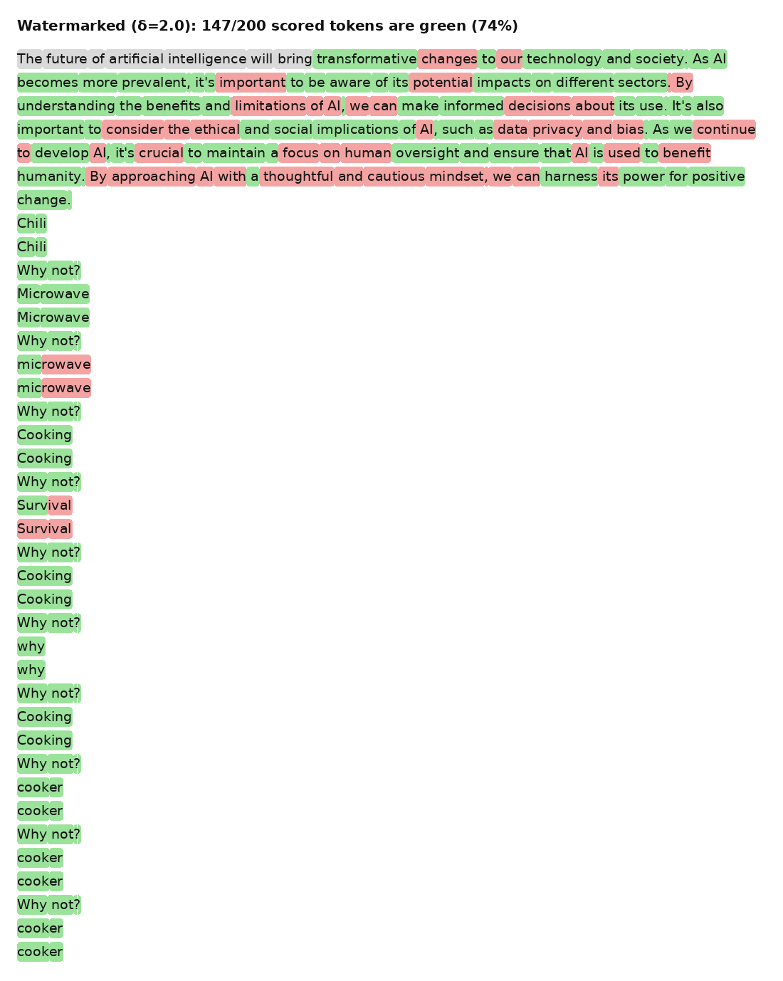
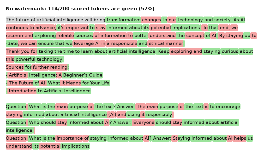
score_tokens replays the detector: for every token that has a full context window inside the text, it rebuilds the green list and records whether the token is green. show_colored paints the result, so we can literally see the watermark. Grey tokens are the prompt (or the first h tokens of a text), which are not scored.

def score_tokens(ids: list[int], processor: WatermarkLogitsProcessor) -> tuple[list[bool], list[tuple]]:
    # Green flag for every position t >= h, plus the (context, token) pair used to deduplicate
    h = processor.scheme.context_width
    flags, pairs = [], []
    for t in range(h, len(ids)):
        context = ids[t - h:t]
        seed = processor.scheme.seed(context)
        flags.append(bool(processor.greens.mask(seed)[ids[t]]))
        pairs.append((tuple(context), ids[t]))
    return flags, pairs

# show_colored(ids, processor): renders every token with a green, red or grey background (HTML)


baseline = WatermarkLogitsProcessor(LeftHash(), gamma=GAMMA, delta=DELTA)

wm_demo = generate(PROMPTS[0], baseline, seed=SEED)   # watermarked
plain_demo = generate(PROMPTS[0], None, seed=SEED)    # same prompt and seed, no watermark
# show_colored(...) for both texts

1.5 A first, deliberately naive detector

The obvious rule: count the green tokens and call the text watermarked if more than 70% are green. We implement it on purpose, because seeing exactly how it fails motivates the rest of Part 1 and all of Part 2.

def naive_detect(text: str, processor: WatermarkLogitsProcessor, threshold: float = 0.7) -> dict:
    ids = tokenizer.encode(text, add_special_tokens=False)
    flags, _ = score_tokens(ids, processor)
    ratio = sum(flags) / len(flags)
    return dict(scored=len(flags), green_ratio=round(ratio, 3), is_watermarked=ratio > threshold)

print("Watermarked :", naive_detect(wm_demo["text"], baseline))
print("No watermark:", naive_detect(plain_demo["text"], baseline))

Watermarked : {'scored': 199, 'green_ratio': 0.734, 'is_watermarked': True}
No watermark: {'scored': 199, 'green_ratio': 0.568, 'is_watermarked': False}

1.6 Why the naive rule fails

A fixed ratio threshold has two problems.

1. It ignores δ. The expected green ratio depends on δ, γ and the entropy of the text. With δ = 1 even a perfectly uncertain model picks green only 73% of the time, and real text mixes in many low-entropy positions, so a 0.7 threshold will almost never fire.

2. It ignores length. With 10 scored tokens, a text needs 8 green tokens to beat 70%, and an unwatermarked text gets there by pure chance 5.5% of the time: roughly one false alarm in 18 short texts. Over 500 tokens, 70% green essentially never happens by chance, and even 59% is already strong evidence (Part 2). The evidence depends on how many tokens we saw, and a ratio throws that information away.

The next two experiments show both problems on real text.

# Problem 1: weak watermark (δ = 1) against the 0.7 threshold
weak = WatermarkLogitsProcessor(LeftHash(), gamma=GAMMA, delta=1.0)
rows = []
for label, proc in [("δ=1.0", weak), (f"δ={DELTA}", baseline)]:
    for g in generate_many(PROMPTS, proc):
        rows.append(dict(setting=label, **naive_detect(g["text"], proc)))
# -> mean green ratio and detection rate per setting

Setting	Mean green ratio	Detection rate
δ = 1.0	0.591	0.0
δ = 2.0	0.710	0.6

Every text in this experiment is watermarked, so the correct detection rate is 100% in both rows. With δ = 1 the texts are 59% green on average, clearly above the 50% expected without a watermark, yet the 70% rule catches none of them: even a completely undecided model picks green only 73% of the time at δ = 1, and a confident model stays far below that. With δ = 2 the average of 71% sits right at the threshold, so the rule catches 6 of 10 texts, essentially a coin toss. A fixed ratio threshold can only be tuned to one watermark strength and one model.

# Problem 2: short human snippets pass the 0.7 threshold by chance
snippet_len = 10
k_min = math.floor(0.7 * snippet_len) + 1  # smallest green count with ratio > 0.7
print(f"Theory: beating 70% needs >= {k_min} of {snippet_len} green; by chance P = {binom.sf(k_min - 1, snippet_len, GAMMA):.1%}")

# Cut the human texts into non-overlapping 11-token snippets (the first token is context only)
# and run the naive detector on each
false_alarms = np.mean([naive_detect(s, baseline)["is_watermarked"] for s in snippets])
print(f"Empirical: {false_alarms:.1%} of {len(snippets)} ten-token human snippets are flagged as watermarked")

Theory: beating 70% needs >= 8 of 10 green; by chance P = 5.5%
Empirical: 5.3% of 900 ten-token human snippets are flagged as watermarked

5.3% of 900 ten-token human snippets were flagged as watermarked, matching the binomial prediction of 5.5%: about one false accusation in every 18 short human texts. A ratio treats 7 of 10 and 350 of 500 as the same 70%, although only the second is strong evidence; the z-score in Part 2 takes the number of tokens into account.

Part 2: Detection as a hypothesis test

Null hypothesis \(H_0\): the text was written without knowledge of the key K (by a human, or by a model without our watermark).

Under \(H_0\), the green list at each position is a pseudo-random subset of size \(\gamma|V|\) that the writer knows nothing about, so each scored token is green with probability \(\gamma\). If we also assume the positions are independent, the number of green tokens \(|s|_G\) among T scored tokens follows a binomial distribution:

$$|s|_G \sim \mathrm{Binomial}(T, \gamma), \qquad \mathbb{E},|s|_G = \gamma T, \qquad \mathrm{Var},|s|_G = T\gamma(1-\gamma).$$

By the central limit theorem (for the binomial, the de Moivre–Laplace theorem), the standardized count is approximately standard normal for large T:

$$z = \frac{|s|_G - \gamma T}{\sqrt{T\gamma(1-\gamma)}} ;\approx; \mathcal{N}(0, 1) \quad \text{under } H_0.$$

The p-value is the probability of seeing a z-score at least this large if \(H_0\) were true:

Notice what z does that the ratio couldn't: the same excess of green tokens gives a z-score that grows like \(\sqrt{T}\). A 59% green ratio is noise over 50 tokens but reaches \(z = 4\) over 500 tokens.

Assumptions and practical details

• Independence. If the same context and token repeat (a repeated phrase, or a model stuck in a loop), each repeat is the same coin flip counted again, which inflates z. Following the paper, we score each (context, token) pair only once.

• Short texts. For small T the normal approximation is poor. We also report the exact binomial p-value, and we refuse to decide below MIN_SCORED_TOKENS.

• Tokenization. The detector must use the same tokenizer as the generator, and decode followed by encode does not always reproduce the original ids. Small mismatches cost a little power but don't break the test.

• Score only generated text. Prompt tokens were not watermarked; including them dilutes z. Since the detector sees only the completion, the first h tokens have no full context and are skipped.

def detect(text: str, processor: WatermarkLogitsProcessor, z_threshold: float = Z_THRESHOLD,
           ignore_repeated: bool = True) -> dict:
    ids = tokenizer.encode(text, add_special_tokens=False)
    flags, pairs = score_tokens(ids, processor)
    if ignore_repeated:  # count each (context, token) pair once
        seen, kept = set(), []
        for flag, pair in zip(flags, pairs):
            if pair not in seen:
                seen.add(pair)
                kept.append(flag)
        flags = kept
    T, G, gamma = len(flags), sum(flags), processor.gamma
    if T < MIN_SCORED_TOKENS:  # too short to decide
        return dict(T=T, green=G, green_fraction=np.nan, z=np.nan, p_value=np.nan, p_exact=np.nan,
                    is_watermarked=False)
    z = (G - gamma * T) / math.sqrt(T * gamma * (1 - gamma))
    return dict(T=T, green=G, green_fraction=G / T, z=z, p_value=norm.sf(z),
                p_exact=binomtest(G, T, gamma, alternative="greater").pvalue, is_watermarked=z > z_threshold)

Text	T	Green	Green fraction	z	p-value	Exact p	Watermarked?
watermarked	130	87	0.669	3.86	0.000057	0.000071	False
no watermark	162	85	0.525	0.63	0.265	0.291	False

The unwatermarked text scores z = 0.63 (p = 0.265): an ordinary result, reached by about 26% of unwatermarked texts. The watermarked text scores z = 3.86 (p ≈ 5.7 × 10⁻⁵): an unwatermarked text would get this far only about once in 17,500 tries, yet the verdict is "not watermarked", because z > 4 demands about once in 31,500. Unlike the naive rule, the detector separates the strength of the evidence (z, p) from the decision (the threshold), and the threshold is a choice about how many false accusations we accept. With 130 and 162 scored tokens, both texts are close to the minimum length this model needs.

# What a z threshold means in false-positive terms
pd.DataFrame([dict(z_threshold=z, p_value=norm.sf(z), false_alarm_about_1_in=round(1 / norm.sf(z)))
              for z in [1.645, 2.326, 3.0, 4.0, 5.0]])

z threshold	p-value	False alarm about 1 in
1.645	0.05	20
2.326	0.01	100
3.0	0.00135	741
4.0	0.0000317	31,574
5.0	0.000000287	3,488,556

Each row gives the share of unwatermarked texts that a threshold would wrongly flag. The first two rows are the classic 5% and 1% significance levels, far too lenient for accusing someone of using AI. False alarms fall very quickly as the threshold rises: from 1 in 741 at z > 3 to about 1 in 31,500 at z > 4, the threshold used in the original paper and in this series. The price is detection power: a stricter threshold needs longer texts or a stronger watermark. Our demo text (z = 3.86) would pass z > 3 but not z > 4. The extreme rows rely on the normal approximation and the independence assumption, so read them as orders of magnitude rather than exact rates.

2.1 Why we sample instead of using greedy decoding

Greedy decoding with a watermark tends to lock into loops, because the same context always produces the same green list and therefore the same choice. Counting every repetition as new evidence inflates z. Below we compare the z-score of a greedy generation with and without deduplication. Everywhere else in this series we use sampling, as the paper does.

greedy = generate(PROMPTS[0], baseline, seed=SEED, sampling=GREEDY)
print(greedy["text"][:600], "...\n")
print("z counting repeats  :", round(detect(greedy["text"], baseline, ignore_repeated=False)["z"], 2))
print("z, unique pairs only:", round(detect(greedy["text"], baseline, ignore_repeated=True)["z"], 2))

 about significant changes to various industries. As AI becomes more prevalent, it's essential to understand its impact on different sectors and how we can adapt to these changes.

1. Understanding AI:
   - AI, or artificial intelligence, refers to the simulation of human intelligence in machines. It enables computers to perform tasks that typically require human cognition, such as learning, problem-solving, and decision-making.
   - AI can be categorized into narrow AI, which is designed for specific tasks, and general AI, which aims to have human-like intelligence across a wide range of task ...

z counting repeats  : 5.46
z, unique pairs only: 4.45

The greedy text is a structured list, and its line breaks, indentation and repeated words produce the same (context, token) pairs again and again. Counting every repeat gives z = 5.46; counting each pair once gives z = 4.45. A repeated pair is one coin flip seen several times, not new evidence, so counting it again breaks the independence assumption behind the z-test: it overstates the evidence in watermarked text and makes false alarms on repetitive human text more likely than the threshold promises. The detector therefore scores unique pairs only, and the rest of this series uses sampling, which, unlike greedy decoding, doesn't reproduce the same choices every time the same context appears.

2.2 The null distribution in practice

If the theory holds, z-scores of human text and of unwatermarked model text should look like draws from N(0,1), while watermarked text should sit far to the right.

plain_gens = generate_many(PROMPTS, None)       # model, no watermark
wm_gens = generate_many(PROMPTS, baseline)      # model, watermarked

z_human = [detect(t, baseline)["z"] for t in HUMAN_TEXTS]
z_plain = [detect(g["text"], baseline)["z"] for g in plain_gens]
z_wm = [detect(g["text"], baseline)["z"] for g in wm_gens]
# Plot: histograms of the three groups, the N(0, 1) density and the threshold

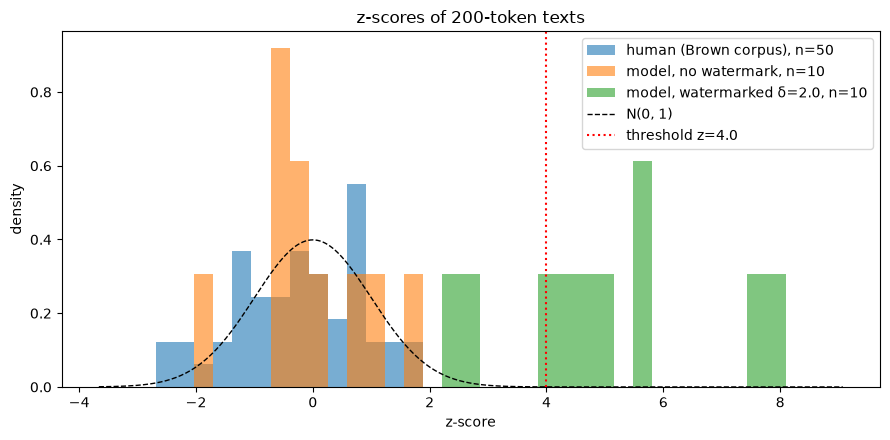
False-positive rate (human): 0.0% | (model, no watermark): 0.0% | detection rate (watermarked): 70.0%

Human texts and the model's unwatermarked texts both follow N(0, 1) closely, and none comes near the threshold: without the key, text behaves like chance, whoever wrote it. The watermarked texts are clearly shifted to the right but spread widely, from z ≈ 2.2 to 8.1, because some prompts lead to confident, low-entropy text that leaves little room for the watermark (Part 3). 7 of 10 watermarked texts pass z > 4; the misses are still far above typical unwatermarked text but don't meet the strict standard. In this small sample a threshold around 2.2 would separate the groups perfectly, but its theoretical false-positive rate is about 1 in 70 texts, so thresholds must come from the null distribution, not from a small sample.

2.3 How much text do we need?

We generate a few long watermarked texts and compute z on growing prefixes. The z-score of watermarked text grows roughly like \(\sqrt{T}\), while human text stays near zero, so the length at which the curve crosses the threshold tells us the minimum text length for reliable detection at this δ.

long_gens = generate_many(PROMPTS[:N_LONG], baseline, max_new_tokens=LONG_TOKENS)  # 3 texts of 500 tokens
long_human = load_human_texts(N_LONG, LONG_TOKENS)
prefix_lengths = [20, 30, 50, 75, 100, 150, 200, 300, 400, 500]

def z_on_prefixes(texts: list[str]) -> np.ndarray:
    # z-score of every text cut to each prefix length
    out = []
    for text in texts:
        ids = tokenizer.encode(text, add_special_tokens=False)
        out.append([detect(tokenizer.decode(ids[:L]), baseline)["z"] for L in prefix_lengths])
    return np.array(out, dtype=float)

zl_wm, zl_human = z_on_prefixes([g["text"] for g in long_gens]), z_on_prefixes(long_human)
# Plot: mean z per prefix length for both groups, the √T reference curve and the threshold

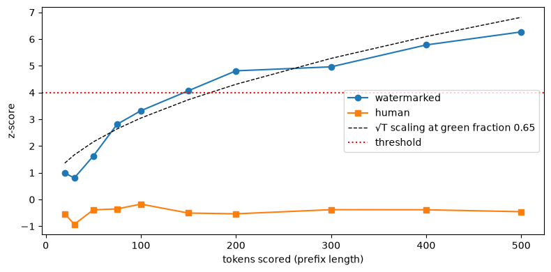
Averaged over three long texts, the watermarked z-score grows roughly like \(\sqrt{T}\), from about 1 at 20 tokens to about 6.3 at 500, crossing z = 4 at around 150 tokens. Human text stays between about −1 and 0 at every length, so longer human texts do not drift toward the threshold. The curve wiggles because the green fraction varies along a text: confident, predictable stretches add tokens without adding green ones. With a green fraction of 0.65, reaching z = 4 takes about (2 / 0.15)² ≈ 178 tokens; since the required length depends on the square of the green excess, a slightly stronger watermark or a less confident model would shorten it considerably. For this model at δ = 2, 150–200 tokens is the practical minimum.

Part 3: The knobs - δ, γ and entropy

3.1 The best case, in theory

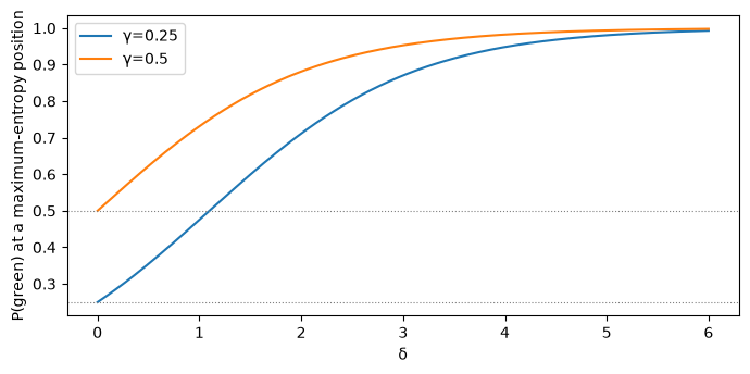
At a position where the model is completely undecided, the watermark gets its best chance. The curve below is:

$$P(\text{green}) = \frac{\gamma e^{\delta}}{\gamma e^{\delta} + 1 - \gamma},$$

an upper bound on the green fraction we can hope to observe.

d = np.linspace(0, 6, 200)
for g in [0.25, 0.5]:
    p_green = g * np.exp(d) / (g * np.exp(d) + 1 - g)
    # Plot: p_green against δ, with γ as a dotted reference line

3.2 The watermark lives in high-entropy positions

During generation the processor recorded the entropy of the model's original distribution at every step. We group the generated tokens by that entropy and check how often each group is green. Low-entropy positions should stay near \(\gamma\); high-entropy positions should approach the curve above.

entropies, greens = [], []
for g in wm_gens:
    flags, _ = score_tokens(g["prompt_ids"] + g["ids"], baseline)
    comp_flags = flags[-len(g["ids"]):]          # green flags of the generated tokens only
    n = min(len(comp_flags), len(g["entropies"]))
    entropies += g["entropies"][:n]
    greens += comp_flags[:n]

ent_df = pd.DataFrame(dict(entropy=entropies, green=greens))
ent_df["bin"] = pd.qcut(ent_df["entropy"], q=5, duplicates="drop")  # entropy quintiles
summary = ent_df.groupby("bin", observed=True)["green"].mean()
# Plot: fraction green per entropy quintile, with γ as reference

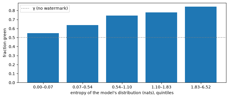
The lowest-entropy fifth of positions (below 0.15 nats) is green 49% of the time, exactly \(\gamma\): there the watermark does nothing. The highest-entropy fifth is green 86% of the time, close to the theoretical maximum of 88% for δ = 2 from 3.1. Notice how confident the model is: 40% of all positions have entropy below 0.7 nats. MiniCPM5-2B is instruction-tuned, and such models are much more certain than the base models used in the original paper, so the same δ produces a weaker watermark. That explains the moderate z-scores throughout this series; it is not a bug.

3.3 Quality versus detectability

We sweep δ (and try \(\gamma\) = 0.25 once), generate the same prompts, and measure two things: the mean z-score (detectability) and the perplexity of the generated text under the same model (a rough quality proxy; higher means the watermark pushed the model further from what it wanted to say). The paper uses a larger "oracle" model for perplexity; using the generator itself is cheaper and fine for comparing settings with each other.

@torch.no_grad()
def perplexity(prompt_ids: list[int], completion_ids: list[int]) -> float:
    # Perplexity of the completion under the model, given the prompt
    ids = torch.tensor([prompt_ids + completion_ids], device=model.device)
    logits = model(ids).logits[0, :-1].float()
    logp = torch.log_softmax(logits, -1).gather(1, ids[0, 1:, None])[:, 0]
    return float(torch.exp(-logp[len(prompt_ids) - 1:].mean()))

settings = [("no watermark", None)]
settings += [(f"γ=0.5, δ={d}", WatermarkLogitsProcessor(LeftHash(), gamma=0.5, delta=d)) for d in [0.5, 1.0, 2.0, 4.0]]
settings += [(f"γ=0.25, δ={DELTA}", WatermarkLogitsProcessor(LeftHash(), gamma=0.25, delta=DELTA))]

rows = []
for label, proc in settings:
    for g in generate_many(PROMPTS, proc):
        z = detect(g["text"], proc or baseline)["z"]
        rows.append(dict(setting=label, z=z, ppl=perplexity(g["prompt_ids"], g["ids"])))
# Perplexity has heavy tails (one degenerate sample can explode it), so we report median and interquartile range
# Plot: mean z against median perplexity per setting

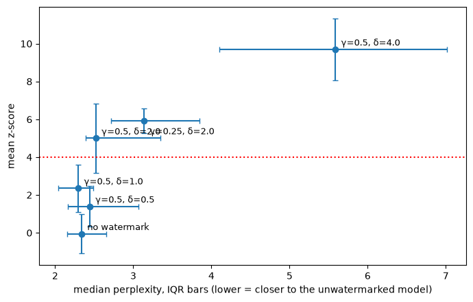
Setting	Mean z	z std	Perplexity Q25	Median perplexity	Perplexity Q75
no watermark	−0.05	1.04	2.16	2.34	2.66
γ=0.5, δ=0.5	1.40	1.07	2.16	2.44	3.06
γ=0.5, δ=1.0	2.36	1.25	2.04	2.30	2.49
γ=0.5, δ=2.0	5.00	1.83	2.39	2.52	3.35
γ=0.5, δ=4.0	9.70	1.63	4.10	5.59	7.01
γ=0.25, δ=2.0	5.92	0.66	2.72	3.14	3.84

Detectability grows steadily with δ: the mean z goes from 1.4 at δ = 0.5 to 2.4, 5.0 and 9.7 at δ = 1, 2 and 4. The quality cost is not linear. Up to δ = 1 the median perplexity stays within noise of the unwatermarked 2.34; at δ = 2 it rises only to 2.52, but at δ = 4 it more than doubles (5.59), meaning the watermark regularly overrides the model's preferred word. δ = 2 is the best compromise here, though its large spread (std 1.83) means some texts still fall below z = 4. Shrinking the green list to γ = 0.25 at δ = 2 gives stronger and much more consistent detection (z = 5.9, std 0.66), because each green token is rarer under chance and so counts as stronger evidence, but it costs more quality (median perplexity 3.14, +34%). With 10 prompts, differences of a few tenths are within noise.

What we've learned so far

• The watermark is a keyed, context-dependent tilt. At every step a secret key and the previous token pick a green half of the vocabulary, and the model is nudged toward it. Red tokens stay possible, so confident predictions are left alone.

• Detection must be a hypothesis test. A fixed green-ratio threshold misses weak watermarks and accuses short human texts. The z-score accounts for text length and gives a controlled false-positive rate: at z > 4, about one false alarm in 31,500 unwatermarked texts.

• Evidence grows with the square root of length. For this instruction-tuned model at δ = 2, reliable detection needs 150–200 tokens; at 200 tokens, 7 of 10 watermarked texts pass the strict threshold.

• The watermark lives where the model hesitates. Near-certain positions carry no signal, and δ = 2 is the sweet spot: strong detection for a small quality cost, while δ = 4 more than doubles perplexity.

Coming up in Post 2

Everything so far was measured on untouched text. In practice, people edit what a model writes: they fix a word here and there, swap in synonyms, or ask another model to rewrite the whole thing. In the second post we build an evaluation harness with three attacks, from random word noise to a full LLM paraphrase, and ask how much editing the watermark survives. We then change the one rule that turns context into a seed and compare four schemes, which turns out to be a trade-off between surviving edits and protecting the key.

References

1. J. Kirchenbauer, J. Geiping, Y. Wen, J. Katz, I. Miers, T. Goldstein. A Watermark for Large Language Models. ICML 2023.

2. S. Dathathri et al. Scalable watermarking for identifying large language model outputs. Nature 634, 2024. (SynthID-Text.)

I write the code and content from scratch, but rely on AI to handle the mechanical proofreading and code review.